
Creating the big-data datasets
In this four-part series of articles, we take you through the development of the Business Risk Index – one of the most complex projects ever undertaken at CreditorWatch.
In my first article I outlined how we built the master datasets and our online transaction processing platform (OLTP), which fuels our data analysis and most of the CreditorWatch’s website and platform. In this article, we’ll cover how we architected and built our online big data analytics process platform (OLAP) and the steps we’ve taken to be able to process a vast amount of data in a quite small timeframe.
Creating the raw datasets
The first step is to create periodic database extracts from (mostly) MySQL databases to our data lake in Parquet1 format.
Our Risk Rating (a predictive company credit score) and Payment Rating (based on a company’s payment history) metrics and the Business Risk Index are built once a month, but the extracts are performed every day to guarantee the freshness of the data for some daily and weekly reports that use data from the OLTP platform. Our data lake is then, our de facto reporting database, which is an absolute must in a Microservice Architecture2.
To perform such extracts, we use AWS’ Database Migration Services (AWS DMS) which collect the data from the source databases in our OLTP platform, transform it to Parquet format and drop it into our S3 data lake. We chose Parquet for its compression, performance and its widespread adoption and support in the Big Data community.
Defining the dataset
The Business Risk Index is the combination of the Risk Rating dataset, the Payment Rating dataset and some extra data from the Australian Bureau of Statistics (ABS). The ABS data is downloaded in CSV format every time there’s an update and is in the data lake already.
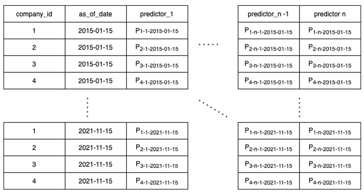
Risk Rating and Payment Rating are built in a similar fashion. A more detailed process will be featured in the next article so, for now, the most important thing to know is that the dataset is a collection of predictors for each company for each date and that these predictors are used for training purposes and to, once the dataset is trained, generate the final Risk Rating and Payment Rating.
The number of predictors keeps growing in every iteration and at the time of writing this article it is near 200 for Risk Rating alone, which means that, with close to 20 million companies and over seven years (84 months), the Risk Rating dataset alone is 336 billion datapoints.
A predictor can be, for instance, the number of officeholders of a company in a specific point of time, or how late on average they were paying their bills at a specific point in time.
Building the dataset
To process and calculate all this data, we use Apache Spark3. Apache Spark is a distributed processing engine for big data and machine learning that allows us to reliably process and compute all these predictors in a simple way just by coding them in SQL.
For the language, R and Python indistinctively, since all the logic is coded in SQL, making the language just the container of the logic, which is implemented in SQL. This allows us to be more portable and be able to change from R to Python at will quite easily in this phase.
Also, while data scientists and data engineers might be more familiar with raw R or Python, most engineers know SQL well. This decision-making and approach allows any engineer in our organisation not only to be able to comfortably read the logic of those predictors and make better decisions based of it, but to create their own if they need it with the skillset they have.
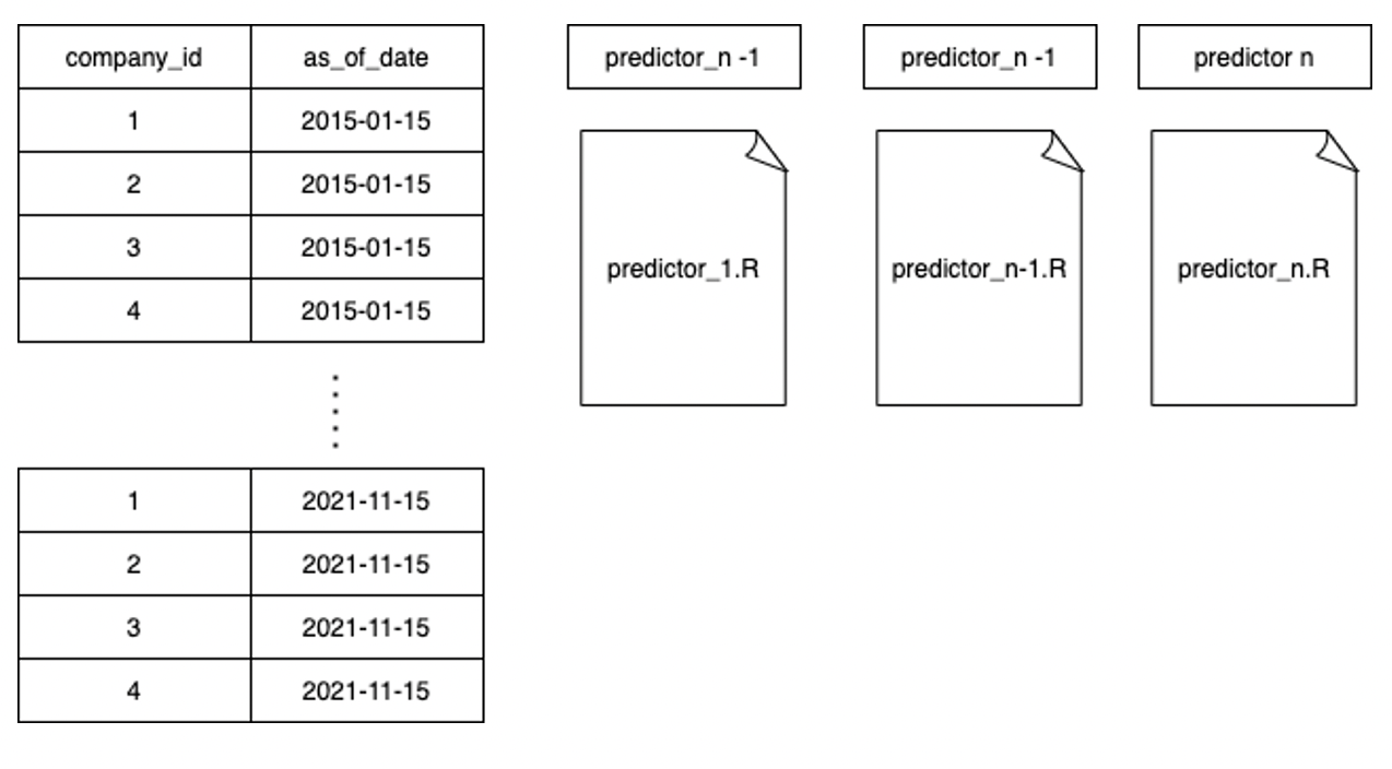
To develop the predictors, we use one file per predictor or family of predictive models. This is a very important part of our SDLC (Software Development Lifecycle), since once that file is tested, approved, peer-code reviewed and documented, the predictive analytics can’t be modified again unless we find a bug.
This ensures that the meaning of that predictor doesn’t change over time and that new bugs are not accidentally introduced as part of other lines of work from other developers. It also allows several developers to work in different predictors in parallel, since it creates no dependencies between different predictors and increases optimization.
Going a bit deeper, predictor_i.R is actually two files: a function file and a script file:
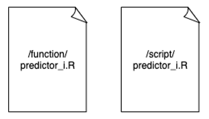
The script files contain all the server-specific configuration and the routes and pointers to the datasets, while the function file contains the SQL logic that would run in any environment. This allows us to switch Spark clusters and configurations entirely. At the time of writing this article, we have executed this approach using an on-premises, data integration cluster, AWS’ Elastic Map Reduce (EMR) and Databricks. The only difference between all three is the script files. The logic, which shouldn’t change based on the environment it runs, never needs to be touched.
Now that we have all the files that generate all the predictors, we need to run all these files in a pipeline. There are many pipeline orchestrators out there – Airflow probably the most popular at the moment. We use Jenkins and Blue Ocean, mainly because all our developments are currently in Jenkins, and it provides a centralised platform for our data management deployments.
Regardless of the technology used, though, the concept still applies. We need a way to reliably trigger the process of every single predictor and, at the end, when all predictors are calculated, we need a way to merge all those predictors in a single dataset and calculate the complex data of the Risk Score/Payment Predictor/Business Risk Index out of it.
Another great outcome from the way we designed our predictor code is that not only can developers work in parallel, but the execution can be parallelised too. We wrote a detailed article about different pipelines architectures in our tech blog showcasing how different pipeline architectures can help different use cases and efficiency in regard to data processing.
We chose to execute pipelines in parallel (Risk Rating and Payment Predictor) with parallel predictors – each one in one small cluster. This way we could reduce the processing time from several days to a few hours.
One of the biggest advantages of this approach is scalability. We could double the number of predictors and the cost in time of generating all the predictors would be the cost of the slowest one. This means that we can multiply the number of predictors and datapoints and we’d only need to multiply the number of small clusters deployed, keeping the cost in time constant. This is not accidental. As a data company we are constantly and actively searching for more data sources, different types of data and new data points, so it was no secret that the amount of data in our platform would dramatically increase, making this scalability feature (‘-ility’ for the architects) a must in our architecture design.
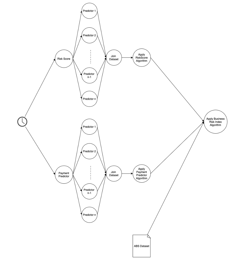
A final snapshot of the BRI pipeline would look like:
So, in summary, we have:
- Created the master dataset via DMS tasks and events from our event-driven architecture and the master dataset lives in our Data Lake
- Used Spark, S3 and Parquet files to create our datasets
- Created two files for each predictor or family of predictors: a configuration one and a logic one
- Generated pipelines that execute all predictors in parallel, join the dataset and apply certain algorithms (Risk Rating or Payment Predictor) to such datasets.
- Ensured that each predictor spins up (and down) its own Spark cluster so the processing time remains constant for each predictor
- Executed each pipeline in parallel
- Once all the pipelines are finished, we gather the datasets and ABS data and execute the Business Risk Index algorithm.
In the next article, I’ll cover in more detail the Risk Rating, Payment Predictor and Business Risk Index algorithms from a data science point of view. I’ll also outline how we choose the predictors that go into the high volume models in a generic way and how predictors are used to generate the final datasets.
Sources:
[1] https://parquet.apache.org/documentation/latest/
[2]Sam Newman. 2015. Building Microservices (1st. ed.). O’Reilly Media, Inc.